Article - Physically Based Rendering - Cook–Torrance

Introduction

In this article we will explore and understand the application of the Cook-Torrance BRDF in a physically based model. I assume that you are familiar with the ideas presented in the previous article Physically Based Rendering; if not, please consider starting from there before approaching this more advanced topic.

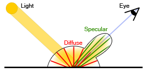
Cook-Torrance BRDF is a function that can be plugged into the rendering equation as \(f_r\). With this BRDF we model the behaviour of light in two different ways making a distinction between diffuse reflection and specular reflection. The idea is that the material we are simulating reflects a certain amount of light in all directions (Lambert) and another amount in a specular way (like a mirror). Because of this the Cook-Torrance BRDF doesn't completely replace the one we have previously but instead, with this new model, we will be able to specify how much radiance is diffused and how much is reflected in a specular way depending on what material we are trying to simulate. The BRDF function \(f_r\) looks like this:

Where \(f_{lambert}\) describes the diffuse component, \(f_{cook-torrance}\) describes the specular component, \(k_d\) is the amount of incoming radiance that gets diffused and \(k_s\) is the amount of light that is specularly reflected. If a given material exhibits a strong diffusive behaviour we have a high value for \(k_d\), while if it behaves more like a mirror we will have high \(k_s\).

It's important to notice that realistic materials shouldn't reflect more energy than they are receiving, which means that the sum of all the BRDF weights across the hemisphere has to be smaller or equal to one, which we write as \( \forall \omega_i \int\limits_{\Omega} f_r  (n \cdot \omega_o) d\omega_o \leq 1\). We can read the formula as "for all incoming light rays the sum of all the outgoing brdf weights multiplied by the cosine of the angle must be smaller or equal to one". If the result is greater than one then the surface would be emitting energy (like a light source) which is something we don't want for a non emissive material. Also, to guarantee the energy conservation we will enforce that \(k_d +  k_s \leq 1\).

Cook-Torrance BRDF

We know from the previous presentation that \(f_{lambert} = \frac{c}{\pi}\), so the last ingredient we need to fully define \(f_r\) is \(f_{cook-torrance}\) that we define as follow:

\[f_{cook-torrance} = \frac{DFG}{4(\omega_o \cdot n)(\omega_i \cdot n)} \]

Where \(D\) is the distribution function, \(F\) is the fresnel function and \(G\) is the geometry function. These three functions are the backbone of the Cook-Torrance model and each one tries to model a specific behaviour of the surface's material we are trying to simulate. The approximation model of the surface that Cook and Torrance have used falls into the category of the Microfacet models which revolves around the idea that rough surfaces can be modelled as a collection of small microfacets. These microfacets are assumed to be very small perfect reflectors and their behaviour is described by statistical models, and in our case both functions \(D\) and \(G\) are based on this idea.

The distribution function \(D\) is used to describe the statistical orientation of the micro facets at some given point. For example if 20% of the facets are oriented facing some vector m, feeding m into the distribution function will give us back 0.2. There are several functions in literature to describe this distributions (such as Phong, or Beckmann) but the function that we will use for our distribution will be the GGX [1] which is defined as follow:

\[ \chi(x) = \cases{ 1 & \text{if } x > 0\cr 0 & \text{if } x \le 0 } \]

\[D(m,n,\alpha)=\frac{\alpha^2\chi(h \cdot n)}{\pi( (m \cdot n)^2(\alpha^2+tan^2(\theta_m))^2}=\frac{\alpha^2\chi(h \cdot n)}{\pi( (m \cdot n)^2(\alpha^2+(\frac{1-(m \cdot n)^2}{(m \cdot n)^2}))^2}\]

Where \(\alpha\) is the roughness of the surface (range [0,1]) and \(m\) is the direction vector that want to check.

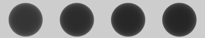
The function using as input the half vector and an array of different roughness values looks like this:

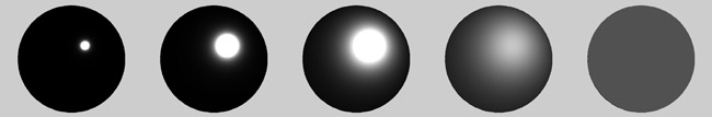
GGX Distribution: From left to right roughness is 0.1, 0.3, 0.6, 0.8, 1.0

As you can see when the roughness is low (leftmost image) only a few points are oriented towards the half vector, but within those points a great quantity of microfacets are oriented that way and this is represented by the white output. When the roughness is higher more and more points have some percentage of microfacets oriented the same way of the half vector, within those points there are only a handful of microfacets oriented the right way and this is represented by the gray colour. The HLSL code reads as follow:

float chiGGX(float v)
{
    return v > 0 ? 1 : 0;
}

float GGX_Distribution(float3 n, float3 h, float alpha)
{
    float NoH = dot(n,h);
    float alpha2 = alpha * alpha;
    float NoH2 = NoH * NoH;
    float den = NoH2 * alpha2 + (1 - NoH2);
    return (chiGGX(NoH) * alpha2) / ( PI * den * den );
}

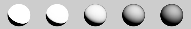
The geometry function \(G\) is used to describe the attenuation of the light due to the microfacets shadowing each other. This is a statistical approximation again and it models the probability that at a given point the microfacets are occluded by each other or that light bounces on multiple microfacets, loosing energy in the process, before reaching the observer's eye. The geometry attenuation is derived from the distribution function so our \(G\) is paired with the GGX \(D\):

\[G(\omega_i,\omega_o,m,n,\alpha)=G_p(\omega_o,m,n,\alpha)G_p(\omega_i,m,n,\alpha)\]

\[G_p(\omega,m,n,\alpha)=\chi(\frac{\omega \cdot m}{\omega \cdot n}) \frac{2}{1 + \sqrt{1 + \alpha^2 \frac{1 - (\omega \cdot m)^2}{(\omega \cdot m)^2} } } \]

 

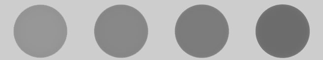
GGX Geometry: From left to right roughness is 0.0, 0.2, 0.5, 0.8, 1.0

The HLSL code for the partial geometry term \(G_p\):

float chiGGX(float v)
{
    return v > 0 ? 1 : 0;
}

float GGX_PartialGeometryTerm(float3 v, float3 n, float3 h, float alpha)
{
    float VoH2 = saturate(dot(v,h));
    float chi = chiGGX( VoH2 / saturate(dot(v,n)) );
    VoH2 = VoH2 * VoH2;
    float tan2 = ( 1 - VoH2 ) / VoH2;
    return (chi * 2) / ( 1 + sqrt( 1 + alpha * alpha * tan2 ) );
}

The fresnel function \(F\) is used to simulate the way light interacts with a surface at different angles. The function accepts in input the incoming ray and a few surface's proprieties. The actual formula is rather complex and is different for conductive and dielectrics materials, but there is a nice approximated version presented by Shlick C. (1994) that can be evaluated very quickly and that we will use for our model (on dielectric materials):

\[ F = F_0+(1-F_o)(1-cos(\theta))^5\]

\[F_0 = (\frac{\eta_1-\eta_2}{\eta_1+\eta2})^2 \]

Where \(\theta\) is the angle between the viewing direction and the half vector while the parameters \(\eta_1\) and \(\eta_2\) are the indices of refraction (IOR) of the two medias. This formula is an approximation of the full version that describes the interaction of light passing from dielectric to dielectric materials with different index of refraction. If we want to model conductor materials we have to use a different formula though. A good approximation for conductors is given by the following [2]:

\[ F = \frac{(\eta-1)^2+4\eta(1-cos\theta)^5+k^2}{(\eta+1)^2+k^2}\]

Where \(\theta\) is the angle between the viewing direction and the half vector, \(\eta\) is the index of refraction for the conductor and \(k\) is the absorption coefficient of the conductor. The formula assumes the media where the ray is coming from is air or vacuum.

 

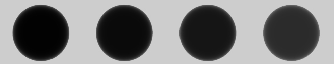
Dielectric Fresnel: From left to right the index of refraction is 1.2, 1.5, 1.8, 2.4

 

Conductor Fresnel with Absorption k = 2: From left to right the index of refraction is 1.2, 1.5, 1.8, 2.4

 

Conductor Fresnel with Absorption k = 4: From left to right the index of refraction is 1.2, 1.5, 1.8, 2.4

 

As you can see above the two function give very different results and depending of what material we are trying to simulate we would have to pick one formula or the other. We could use the formulas as presented, but the current trend, used by the top notch engines like Unreal, is to approximate even more using a concept introduced in the Cook-Torrance paper: the idea of reflectance at normal incidence. To keep the math simple the idea is to precalculate the material's response at normal incidence and then interpolate this value based on the view angle. This is also based on Schlick's approximation:

float3 Fresnel_Schlick(float cosT, float3 F0)
{
  return F0 + (1-F0) * pow( 1 - cosT, 5);
}

Where F0 is the material's response at normal incidence. We calculate F0 as follow:

// Calculate colour at normal incidence
float3 F0 = abs ((1.0 - ior) / (1.0 + ior));
F0 = F0 * F0;
F0 = lerp(F0, materialColour.rgb, metallic);

The last line is a trick that allows us to treat conductors and dielectric with the same approximation. The idea is that if the material is dielectric we use the IOR, otherwise we use the albedo colour to "tint" the reflection. This can be a bit confusing, especially when authoring the assets, so the important thing to remember is that with this implementation we ignore the IOR value if metallic is set to 1, and we use the albedo colour instead.

Cook-Torrance

We now have all the pieces of our formula, and we can put them together to complete our BRDF which now reads as follow:

\[f_r = k_d \frac{c}{\pi} + k_s \frac{DFG}{4(\omega_o \cdot n)(\omega_i \cdot n)} \]

As presented in the previous article Physically Based Rendering the BRDF is plugged into the rendering equation which is then approximated via a Monte Carlo algorithm. We have also seen how to precalculate the integral result and store it into an envmap; unfortunately this approach won't be possible with Cook-Torrance's BRDF, because it depends on two vectors instead of only one. This means that we won't be able to precalculate it and we'll have to solve it every frame.

• One is to save inside the envmap part of the formula convolved with the actual radiance map; this will also take advantage of the lower mips of the envmap.
• The second one is to use importance sampling instead of Monte Carlo vanilla.

It could easily take another article per technique in order to properly explain how we derive them and why, but here I will simply present the final result with a few hints on how we got there. Also, we will limit ourselves to use the mip levels without any prefiltering, which is a bit hacky but reduce the number of samples we need during the importance sampling pass.

Importance sampling

Importance sampling substantially improves the Monte Carlo algorithm by introducing a guided approach to the sampling. The idea is that we can define a probability distribution function that describes where we want to sample more and where we want to sample less. This has several implications that change the Monte Carlo formula a bit, but unfortunately we won't have the time to see this as it would be quite long. Let's just define the new estimator when using importance sampling as follows:

\[\hat{f}(x)=\frac{1}{N}  \sum_{i=1}^{N} \frac{f(x)}{p(x)} \]

For GGX we use the following function for the probability: \(p(h,n,\alpha)=D(h,n,\alpha)|h \cdot n|\). Also, we now run the estimator some N times, but what input do we feed to the function? Previously we were scanning the hemisphere in a discreet fashion, but now we sample only in the "important" areas, so how do we generate the correct vectors? The full derivation of the method of generating the sampling vectors is quite long (but worth learning, especially if you want to play with your own probability functions) so for this article we will simply use the following angles without proving out why:

\[\theta_s = arctan(\frac{\alpha\sqrt{\xi_1}}{\sqrt{1-\xi_1}})\]

\[\phi_s = 2\pi\xi_2\]

Where \(\theta_s\) is the theta angle of the vector we need for sampling, and \(\phi_s\) is the phi angle. The variables we need to obtain these two angles are \(\xi_1\) and \(\xi_2\) which are two uniform randomly generated variables in the range [0,1].

Final Steps

We are finally there, we can now put together the whole thing into an actual usable formula:

\[k_s \int\limits_{\Omega} \frac{DFG}{4(\omega_o \cdot n)(\omega_i \cdot n)}) L_i(p,\omega_i) (\mathbf n \cdot \omega_i) d\omega_i \approx k_s \frac{1}{N} \sum_{i=1}^{N} \frac{L_i(\omega_i,p)F(\eta_i,\eta_t,h,\omega_o)G(\omega_i,\omega_o,h,n)sin(\theta_i)}{4|\omega_o \cdot n||h \cdot n|} \]

That in code we translate to something like this:

By using this Monte Carlo estimator we can evaluate how much light is reflected by the surface and we can then add it to the diffuse component that we have calculated using Lambert. The last thing we need now is to calculate the two weights \(k_d\) and \(k_s\). Since these weights represent the amount of light reflected it's natural to immediately think of fresnel. In fact we can use fresnel itself for \(k_s\) and then, for the energy conservation law, we can derive \(k_d\) as \(k_d=1-k_s\). It's important to notice that in the GGX calculation we have already multiplied the radiance by fresnel, so in the final formula we won't be doing it again.

Also, note that \(k_d\) is weighted by (1-metallic). This is to simulate the fact that a metallic surface doesn't diffuse light at all, so it can't have a diffuse component.

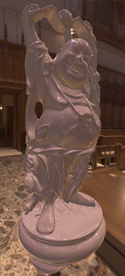
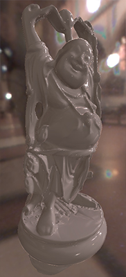
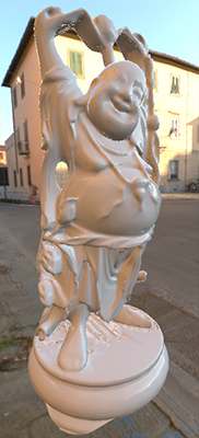
The final results can be seen in the images below. This is the model lit in different lighting conditions:

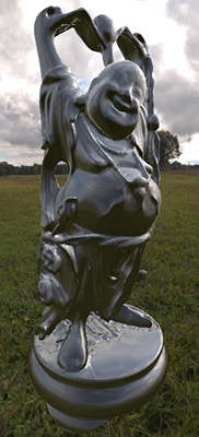
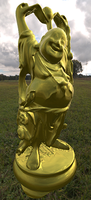
This is the same model with different metallic values (no metal, steel, gold):

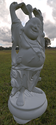
And finally same model with different IOR and roughness values (no specular, rough specular, and glossy specular):

References

[1] Walter et al. "Microfacet Models for Refraction through Rough Surfaces"
[2] Lazanyi, Szirmay-Kalos, “Fresnel term approximations for Metals”